주) 본인 학습을 위해 학습기간중 지속적으로 update 됩니다. 방문하신 분들을 위한 것이 아닙니다. 타이핑 연습용!^^
| 변수유형 | 설명 | 사례 |
| 범주 | 모집단을 독립적인 MECE 분해 ** R에서는 factor라함 |
남녀, 지역별, 고객등급 등 |
| 이산 | 정수형 ** R에서는 integer라함 |
-4, -2, 0,1, 2 3,4 .. |
| 연속 | 실수형 ** R에서는 number라함 |
2.5, 4.0, 3.12, .... |
범주형(Categorized) 변수
범주형 1개 요약
더보기
* 도수분포표
- table() # 빈도수
- prop.table() # 상대빈도
- addmargins() # 합계추가
- round( , digit=2) # 소수점이하 두자리
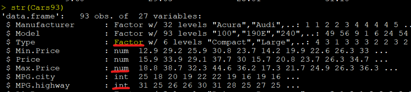
# dataset - MASS - Cars93
library(MASS)
str(Cars93)
# absolute frequency table
table(Cars93$Type)
Compact   Large Midsize   Small  Sporty     Van
     16      11      22      21      14       9
# relative frequency table
prop.table(table(Cars93$Type))
  Compact      Large    Midsize      Small     Sporty        Van
0.17204301 0.11827957 0.23655914 0.22580645 0.15053763 0.09677419
#
addmargins(prop.table(table(Cars93$Type)))

   Compact      Large    Midsize      Small     Sporty        Van        Sum
0.17204301 0.11827957 0.23655914 0.22580645 0.15053763 0.09677419 1.00000000
#
round(addmargins(prop.table(table(Cars93$Type)))*100, digit=2)
Compact   Large Midsize   Small  Sporty     Van     Sum
  17.20   11.83   23.66   22.58   15.05    9.68  100.00
#
# THE END
범주형 2개 요약
더보기
* 분할표, 교차표
- table() # 빈도수
- prop.table() # 상대빈도
- addmargins() # 합계추가
- round( , digit=2) # 소수점이하 두자리
# dataset-MASS-Cars93
library(MASS)
str(Cars93)
df<-Cars93[, c('Origin', 'Type')]
str(df)
'data.frame':   93 obs. of  2 variables:
 $ Origin: Factor w/ 2 levels "USA","non-USA": 2 2 2 2 2 1 1 1 1 1 ...
 $ Type  : Factor w/ 6 levels "Compact","Large",..: 4 3 1 3 3 3 2 2 3 2 ...
# absolute frequency table
table(df)
                       Type
Origin    Compact Large Midsize Small Sporty Van
  USA           7    11      10     7      8   5
  non-USA       9     0      12    14      6   4
# relative frequency table
prop.table(table(df))
                       Type
Origin       Compact      Large    Midsize      Small     Sporty        Van
  USA     0.07526882 0.11827957 0.10752688 0.07526882 0.08602151 0.05376344
  non-USA 0.09677419 0.00000000 0.12903226 0.15053763 0.06451613 0.04301075
addmargins(prop.table(table(df)))
                          Type
Origin       Compact      Large    Midsize      Small     Sporty        Van        Sum
  USA     0.07526882 0.11827957 0.10752688 0.07526882 0.08602151 0.05376344 0.51612903
  non-USA 0.09677419 0.00000000 0.12903226 0.15053763 0.06451613 0.04301075 0.48387097
  Sum     0.17204301 0.11827957 0.23655914 0.22580645 0.15053763 0.09677419 1.00000000
#
round(addmargins(prop.table(table(df)))*100, digit=2)
                          Type
Origin    Compact  Large Midsize  Small Sporty    Van    Sum
  USA        7.53  11.83   10.75   7.53   8.60   5.38  51.61
  non-USA    9.68   0.00   12.90  15.05   6.45   4.30  48.39
  Sum       17.20  11.83   23.66  22.58  15.05   9.68 100.00
#
# THE END
범주형 2개 독립성 검정 - chisq()
더보기
* 독립성 검정
- chisq.test()
- fisher.test()
# independent test
# H0 : 두 변수는 서로 독립니다.
chisq.test(Cars93$Origin, Cars93$Type)
Pearson's Chi-squared test

data:  Cars93$Origin and Cars93$Type
X-squared = 14.08, df = 5, p-value = 0.01511
경고메시지(들):
chisq.test(Cars93$Origin, Cars93$Type)에서:
  카이제곱 approximation은 정확하지 않을수도 있습니다
#
# Fisher exact test
fisher.test(Cars93$Origin, Cars93$Type)
Fisher's Exact Test for Count Data

data:  Cars93$Origin and Cars93$Type
p-value = 0.007248
alternative hypothesis: two.sided
# H0 reject
#
# THE END
연속형(Continuous) 변수
연속형 빈도분포표
더보기
** 연속형변수 구간화(범주화)
예) 월 구매액 기준 고객 등급나누기
남녀별 월 구매액 독립성 검정
- summary # 나눌 구간 확인
- cut(data, c( ,,,,)) # 구간지정
- table(...) # 구간별 빈도수 확인
 summary(Cars93$Price)
   Min. 1st Qu.  Median    Mean 3rd Qu.    Max.
   7.40   12.20   17.70   19.51   23.30   61.90
 table(cut(Cars93$Price, c(5.00,10.00,15.00,20.00,30.00,70.00)))
(5,10] (10,15] (15,20] (20,30] (30,70]
     12      21      29      19      12
#
# THE END
연속형(실수형) 1개 요약
더보기
[출처] 5. 수치형 자료 요약하기1, 통계인재개발원, 2025
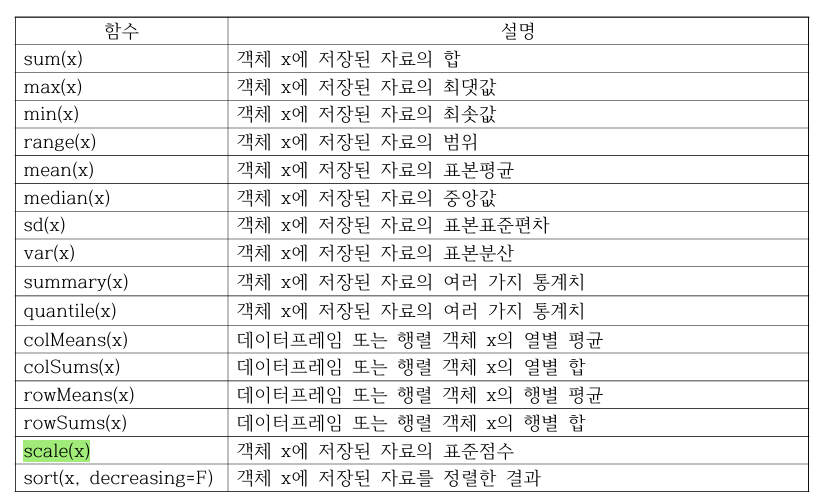
- summary() # 기술통계량
- scale() # 표준화
- quantile() # 사분위
- 일반적인 기술통계량
# dataset - MASS - Cars93
library(MASS)
summary(Cars93$Price)
 Min. 1st Qu.  Median    Mean 3rd Qu.    Max.
7.40   12.20   17.70   19.51   23.30   61.90
# 표준화 평균=0, 표준편차=1
summary(scale(Cars93$Price))
 V1
 Min.   :-1.2537
 1st Qu.:-0.7567
 Median :-0.1873
 Mean   : 0.0000
 3rd Qu.: 0.3924
 Max.   : 4.3885
sd(scale(Cars93$Price))
[1] 1
#
quantile(Cars93$Price)
 0%  25%  50%  75% 100%
 7.4 12.2 17.7 23.3 61.9
# THE END
연속형 1개 분포 검정
더보기
** 정규분포일까?
- ks.test( ) # Kolmogorov-Smirnov test
- shapiro.test( ) # Shapiro-Wilk normality test
# H0: Cars93$Price는 정규분포이다
ks.test(Cars93$Price, 'pnorm')
  Asymptotic one-sample Kolmogorov-Smirnov test

data:  Cars93$Price
D = 1, p-value < 2.2e-16
alternative hypothesis: two-sided

경고메시지(들):
ks.test.default(Cars93$Price, "pnorm")에서:
  ties should not be present for the one-sample Kolmogorov-Smirnov test
# H0 rejected!
#
# shapiro.test(Cars93$Price)
 Shapiro-Wilk normality test

data:  Cars93$Price
W = 0.88051, p-value = 4.235e-07
# H0 rejected
#
# THE END.
'학습 및 사례' 카테고리의 다른 글
| [직접생산확인제도] 한국중소벤처기업유통원 '심사관'은 왜 기준서 내용을 확대 해석하나? (0) | 2025.08.01 |
|---|---|
| [직접생산확인제도] 불분명한 공장 및 신청주소로 인한 '배정업체 반납' 사례(2) (1) | 2025.07.07 |
| Google 제미니와의 컨설팅 협업 - 2차원(=두 변수) 사분면에 기업 배치하기 (0) | 2025.06.15 |
| [빅데이터분석기사 실기 5탄] 학습실행 - 통계분석 (0) | 2025.06.07 |
| [빅데이터분석기사 실기 4탄] 학습실행 - 머신러닝, Unsupervised Learning (0) | 2025.06.02 |